Page 18-59
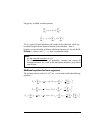
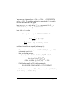
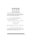
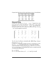
Compare these fitted values with the original data as shown in the table below:
Polynomial fitting
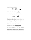
Consider the x-y data set {(x
1
,y
1
), (x
2
,y
2
), …, (x
n
,y
n
)}. Suppose that we want
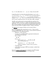
to fit a polynomial or order p to this data set. In other words, we seek a fitting
of the form y = b
0
+ b
1
⋅x + b
2
⋅x
2
+ b
3
⋅x
3
+ … + b
p
⋅x
p
. You can obtain the
least-square approximation to the values of the coefficients b = [b
0
b
1
b
2
b
3
… b
p
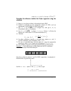
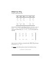
], by putting together the matrix X
__
__
Then, the vector of coefficients is obtained from b = (X
T
⋅X)
-1
⋅X
T
⋅y, where y is
the vector y = [y
1
y
2
… y
n
]
T
.
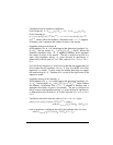
In Chapter 10, we defined the Vandermonde matrix corresponding to a vector
x = [x
1
x
2
… x
m
] . The Vandermonde matrix is similar to the matrix X of
interest to the polynomial fitting, but having only n, rather than (p+1) columns.
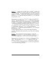
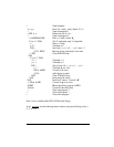
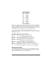
We can take advantage of the VANDERMONDE function to create the matrix X
if we observe the following rules:
If p = n-1, X = V
n
.
If p < n-1, then remove columns p+2, …, n-1, n from V
n
to form X.
x
1
x
2
x
3
yy-fitted
1.20 3.10 2.00 5.70 5.63
2.50 3.10 2.50 8.20 8.25
3.50 4.50 2.50 5.00 5.03
4.00 4.50 3.00 8.20 8.22
6.00 5.00 3.50 9.50 9.45
1x
1
x
1
2
x
1
3
…
x
1
p-1
y
1
p
1x
2
x
2
2
x
2
3
…
x
2
p-1
y
2
p
1x
3
x
3
2
x
3
3
…
x
3
p-1
y
3
p
.... ..
.......
1x
n
x
n
2
x
n
3
…
x
n
p-1
y
n
p


