


Page 16-3
EVAL(ANS(1)) `
In RPN mode:
‘∂t(∂t(u(t)))+ ω0^2*u(t) = 0’ ` ‘u(t)=A*SIN (ω0*t)’ `
SUBST EVAL
The result is ‘0=0’.
For this example, you could also use: ‘∂t(∂t(u(t))))+ ω0^2*u(t) = 0’ to enter the
differential equation.
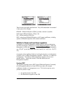
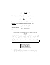
Slope field visualization of solutions
Slope field plots, introduced in Chapter 12, are used to visualize the solutions to
a differential equation of the form dy/dx = f(x,y). A slope field plot shows a
number of segments tangential to the solution curves, y = f(x). The slope of the
segments at any point (x,y) is given by dy/dx = f(x,y), evaluated at any point
(x,y), represents the slope of the tangent line at point (x,y).
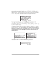
Example 1
-- Trace the solution to the differential equation y’ = f(x,y) = sin x cos
y, using a slope field plot. To solve this problem, follow the instructions in
Chapter 12 for slopefield plots.
If you could reproduce the slope field plot in paper, you can trace by hand lines
that are tangent to the line segments shown in the plot. This lines constitute lines
of y(x,y) = constant, for the solution of y’ = f(x,y). Thus, slope fields are useful
tools for visualizing particularly difficult equations to solve.
In summary, slope fields are graphical aids to sketch the curves y = g(x) that
correspond to solutions of the differential equation dy/dx = f(x,y).
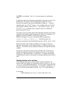
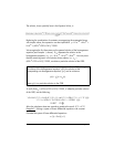
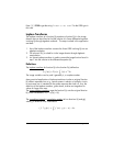
The CALC/DIFF menu
The DIFFERENTIAL EQNS.. sub-menu within the CALC („Ö) menu provides
functions for the solution of differential equations. The menu is listed below with
system flag 117 set to CHOOSE boxes: