Page 18-47
Thus, we accept (more accurately, we do not reject) the hypothesis: H
0
: μ
1
−μ
2
=
0, or H
0
: μ
1
=μ
2
, against the alternative hypothesis H
1
: μ
1
−μ
2
< 0, or H
1
: μ
1
=μ
2
.
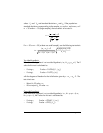
The test t value is t
0
= -1.341776, with a P-value = 0.09130961, and critical t is
–t
α
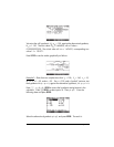
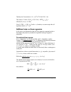
= -1.659782. The graphical results are:
These three examples should be enough to understand the operation of the
hypothesis testing pre-programmed feature in the calculator.
Inferences concerning one variance
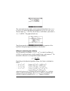
The null hypothesis to be tested is , H
o
: σ
2
= σ
o
2
, at a level of confidence (1-
α)100%, or significance level α, using a sample of size n, and variance s
2
. The
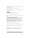
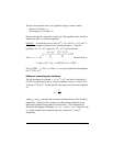
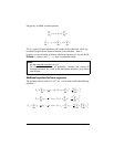
test statistic to be used is a chi-squared test statistic defined as
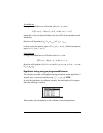
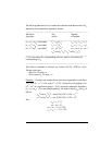
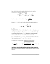
Depending on the alternative hypothesis chosen, the P-value is calculated as
follows:
Θ H
1
: σ
2
< σ
o
2
, P-value = P(χ
2
<χ
o
2
) = 1-UTPC(ν,χ
o
2
)
Θ H
1
: σ
2
> σ
o
2
, P-value = P(χ
2
>χ
o
2
) = UTPC(ν,χ
o
2
)
Θ H
1
: σ
2
≠σ
o
2
, P-value =2⋅min[P(χ
2
<χ
o
2
), P(χ
2
>χ
o
2
)] =
2⋅min[1-UTPC(ν,χ
o
2
), UTPC(ν,χ
o
2
)]
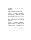
where the function min[x,y] produces the minimum value of x or y (similarly,
max[x,y] produces the maximum value of x or y). UTPC(ν,x) represents the
calculator’s upper-tail probabilities for ν = n - 1 degrees of freedom.
2
0
2
2
)1(
σ
χ
sn
o
−
=


