Page 18-63
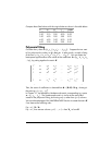
Θ The correlation coefficient, r. This value is constrained to the range –1
< r < 1. The closer r is to +1 or –1, the better the data fitting.
Θ The sum of squared errors, SSE. This is the quantity that is to be
minimized by least-square approach.
Θ A plot of residuals. This is a plot of the error corresponding to each of
the original data points. If these errors are completely random, the
residuals plot should show no particular trend.
Before attempting to program these criteria, we present some definitions
:
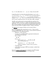
Given the vectors x and y of data to be fit to the polynomial equation, we form
the matrix X and use it to calculate a vector of polynomial coefficients b. We
can calculate a vector of fitted data, y’, by using y’ = X⋅b.
An error vector is calculated by e = y – y’.
The sum of square errors is equal to the square of the magnitude of the error
vector, i.e., SSE = |e|
2
= e•e = Σ e
i
2
= Σ (y
i
-y’
i
)
2
.
To calculate the correlation coefficient we need to calculate first what is known
as the sum of squared totals, SST, defined as SST = Σ (y
i
-⎯y)
2
, where ⎯y is the
mean value of the original y values, i.e., ⎯y = (Σy
i
)/n.
In terms of SSE and SST, the correlation coefficient is defined by
r = [1-(SSE/SST)]
1/2
.
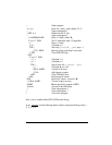
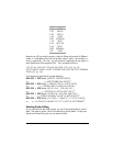
Here is the new program including calculation of SSE and r (Once more,
consult the last page of this chapter to see how to produce the variable and
command names in the program):
« Open program
x y p Enter lists x and y, and number p
« Open subprogram1
x SIZE n Determine size of x list
« Open subprogram 2


