Page 16-50
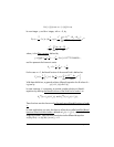
Example 2 – To produce the signal given the spectrum, we modify the program
GDATA to include an absolute value, so that it reads:
<< m a b << ‘2^m’ EVAL n << ‘(b-a)/(n+1)’ EVAL Dx << 1 n FOR j
‘a+(j-1)*Dx’ EVAL f ABS NEXT n ARRY >> >> >> >>
Store this version of the program under GSPEC (Generate SPECtrum). Run the
program with m = 6, a = 0, b = 100. In RPN mode, use:
6#0#100@GSPEC!
Press ` when done, to keep an additional copy of the spectrum array.
Convert this row vector into a column vector and store it into ΣDAT. Following
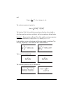
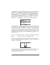
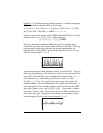
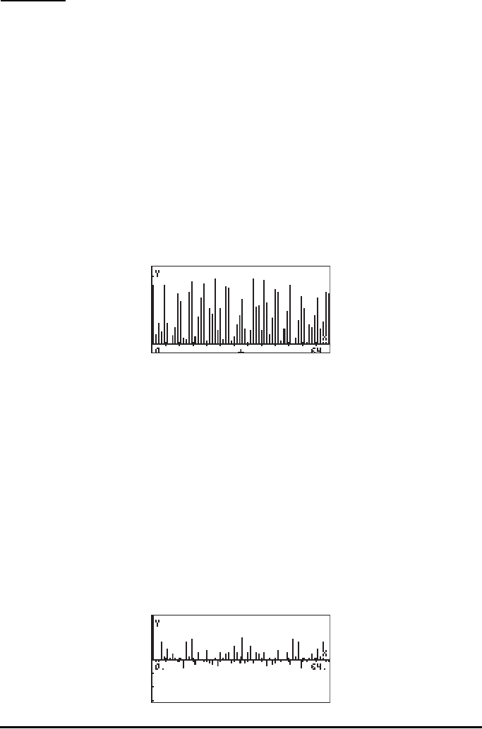
the procedure for generating a bar plot, the spectrum generated for this
example looks as shown below. The horizontal range in this case is 0 to 64,
while the vertical range is –1 to 10:
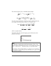
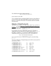
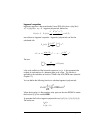
To reproduce the signal whose spectrum is shown , use function IFFT. Since we
left a copy of the spectrum in the stack (a row vector), all you need to do if find
function IFFT in the MTH/FFT menu or through the command catalog, ‚N.
As an alternative, you could simply type the function name, i.e., type
~~ifft`. The signal is shown as an array (row vector) with
complex numbers. We are interested only in the real part of the elements. To
extract the real part of the complex numbers, use function RE from the CMPLX
menu (see Chapter 4), e.g., type ~~re`. What results is another
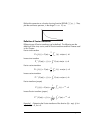
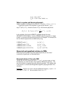
row vector. Convert it into a column vector, store it into ΣDAT, and plot a bar
plot to show the signal. The signal for this example is shown below, using a
horizontal range of 0 to 64, and a vertical range of –1 to 1:


