Page 12-16
„ó
, simultaneously if in RPN mode: Plots the graph based on the settings
stored in variable PPAR and the current functions defined in the PLOT –
FUNCTION screen. If a graph, different from the one you are plotting, already
exists in the graphic display screen, the new plot will be superimposed on the
existing plot. This may not be the result you desire, therefore, I recommend to
use the @ERASE @DRAW soft menu keys available in the PLOT SETUP, PLOT-
FUNCTION or PLOT WINDOW screens.
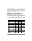
Plots of trigonometric and hyperbolic functions
The procedures used above to plot LN(X) and EXP(X), separately or
simultaneously, can be used to plot any function of the form y = f(x). It is left as
an exercise to the reader to produce the plots of trigonometric and hyperbolic
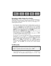
functions and their inverses. The table below suggests the values to use for the
vertical and horizontal ranges in each case. You can include the function Y=X
when plotting simultaneously a function and its inverse to verify their ‘reflection’
about the line Y = X.
H-View range V-View range
Function Minimum Maximum Minimum Maximum
SIN(X) -3.15 3.15 AUTO
ASIN(X) -1.2 1.2 AUTO
SIN & ASIN -3.2 3.2 -1.6 1.6
COS(X) -3.15 3.15 AUTO
ACOS(X) -1.2 1.2 AUTO
COS & ACOS -3.2 3.2 -1.6 1.6
TAN(X) -3.15 3.15 -10 10
ATAN(X) -10 10 -1.8 1.8
TAN & ATAN -2 -2 -2 -2
SINH(X) -2 2 AUTO
ASINH(X) -5 5 AUTO
SINH & ASINH -5 5 -5 5
COSH(X) -2 2 AUTO
ACOSH(X) -1 5 AUTO
COS & ACOS-55-15


